Perron Frobenius Theorem is a well-known algebra result that finds applications in a large span of fields of Mathematics. One can mention Markov chains, population growth (with the Leslie matrix model) or the famous PageRank algorithm. In this post we prove the Perron-Frobenius Theorem for stochastic matrices.
Perron Frobenius Theorem
Let us consider some integer ![]() and
and ![]() a stochastic matrix, meaning that for all
a stochastic matrix, meaning that for all ![]() ,
, ![]() . In the following, we will denote
. In the following, we will denote ![]() . We assume that
. We assume that ![]() is irreducible which means that
is irreducible which means that ![]() Then the period of the point
Then the period of the point ![]() defined by
defined by ![]() does not depend on
does not depend on ![]() meaning that there exists some
meaning that there exists some ![]() such that
such that ![]() . Then:
. Then:
- The spectral radius of
 is
is  . Moreover, the eigenvalues of
  of modulus 1 are exactly the p p-th roots of unity and have algebraic multiplicity of 1.
 - The spectrum of
 is invariant by rotation of angle
  .
. - If
 , it exists a permutation matrix
  such that
where the matrices![Rendered by QuickLaTeX.com \[S^{-1}QS = \begin{bmatrix} 0 & B_{1} & 0 & \dots & 0 \\ 0 & 0 & B_{2} & \dots & 0 \\ \vdots & \vdots & \vdots & \dots &\vdots\\ 0 & 0 & 0 & \dots & B_{p-1}\\ B_{p} & 0 & 0 & \dots & 0 \end{bmatrix},\]](http://quentin-duchemin.alwaysdata.net/wiki/wp-content/ql-cache/quicklatex.com-80cb6e59f2b0e673ce3935439045a664_l3.png)
 are non-zero square matrices.
Proof.
Step 0 : Preliminaries
Let us recall that on a finite state space, an irreducible matrix ![]() has a unique invariant probability distribution
has a unique invariant probability distribution ![]() .
.
Claim 0.1: ![]()
Let us assume that for some ![]() it holds
it holds ![]() . Since
. Since ![]() is a probability measure on a finite space, there exists some
is a probability measure on a finite space, there exists some ![]() such that
such that ![]() . Using that
. Using that ![]() is invariant for
is invariant for ![]() we get directly that
we get directly that ![]() is also an invariant distribution of the matrix
is also an invariant distribution of the matrix ![]() for any
for any ![]() which means that
which means that
![]()
Claim 0.2: Denoting ![]() ,
, ![]() is an irreducible stochastic matrix
is an irreducible stochastic matrix
Claim 0.2 follows from a direct computation using the fact that ![]() is an irreducible stochastic matrix.
is an irreducible stochastic matrix.
Step 1 : Eigenspace associated with the eigenvalue 1
Let us denote ![]() . It is a eigenvector of
. It is a eigenvector of ![]() related to the eigenvalue 1.
related to the eigenvalue 1.
Claim 1.1: The spectral radius of ![]() is 1.
is 1.
Let us denote ![]() an (complex) eigenvalue of
an (complex) eigenvalue of ![]() with the largest modulus and
with the largest modulus and ![]() an non-zero associated eigenvector. Let
an non-zero associated eigenvector. Let ![]() . Since
. Since ![]() , taking the module and using the triangle inequality gives
, taking the module and using the triangle inequality gives
![]()
where the last inequality comes from the fact that ![]() is a stochastic matrix. By definition of
is a stochastic matrix. By definition of ![]() and since
and since ![]() , we have that
, we have that ![]() and the previous inequality leads to
and the previous inequality leads to ![]() . Since 1 is an eigenvalue of
. Since 1 is an eigenvalue of ![]() , we deduce that the spectral radius of
, we deduce that the spectral radius of ![]() is 1.
is 1.
Claim 1.2: For two vectors ![]() , we write
, we write ![]() to state that
to state that ![]() for all
for all ![]() . Then, for any
. Then, for any ![]() such that
such that ![]() and
and ![]() , it holds that
, it holds that ![]() and there exists some
and there exists some ![]() such that
such that ![]() .
.
Let us consider ![]() . Then for any
. Then for any ![]() , we have
, we have
![]()
![]()
Claim 1.3: If ![]() is a complex eigenvector realted to an eigenvalue
is a complex eigenvector realted to an eigenvalue ![]() of modulus 1 of
of modulus 1 of ![]() , then
, then ![]() is an nonnegative eigenvector related to the eigenvalue 1. This implies that the eigenspace related to 1 is
is an nonnegative eigenvector related to the eigenvalue 1. This implies that the eigenspace related to 1 is ![]() .
.
For all ![]() ,
, ![]() . Hence, taking the modulus in the previous inequality and using the triangle inequality leads to
. Hence, taking the modulus in the previous inequality and using the triangle inequality leads to ![]() i.e.
i.e. ![]() Using Claim 1.2, we deduce that
Using Claim 1.2, we deduce that ![]() and that
and that ![]() , which concludes the proof.
, which concludes the proof.
Step 2 : Algebraic multiplicity of the eigenvalue 1
In the following, we will denote ![]() the caracteristic polynomial of the matrix
the caracteristic polynomial of the matrix ![]() and
and ![]() the conjugate of the comatrice of
the conjugate of the comatrice of ![]() . Claim 2.1 is a classical result of differential calculus.
. Claim 2.1 is a classical result of differential calculus.
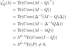
Claim 2.1: ![]() .
.
Claim 2.2: Every column of ![]() belongs to
belongs to ![]() .
.
From Step 1, we know that ![]() has rank
has rank ![]() . Hence
. Hence ![]() and we get that
and we get that
![]()
Claim 2.3: Every line of ![]() is proportional to
is proportional to ![]() .
.
From Step 0, we know that ![]() is an irreducible stochastic matrix and we deduce that this is also the case for
is an irreducible stochastic matrix and we deduce that this is also the case for ![]() . Hence, remarking that Claim 2.2 holds for any irreducible stochastic matrix, we get that every column of
. Hence, remarking that Claim 2.2 holds for any irreducible stochastic matrix, we get that every column of ![]() is proportional to
is proportional to ![]() , meaning that for all
, meaning that for all ![]() , there exists some
, there exists some ![]() such that
such that ![]() for all
for all ![]() where we have denote
where we have denote ![]() the cofactor application related to line
the cofactor application related to line ![]() and column
and column ![]() . Hence, for all
. Hence, for all ![]()
![Rendered by QuickLaTeX.com \begin{align*}a_j&= c_{j,i}(D^{-1}(I-Q^{\top})D) \\ &= \left[Com(D^{-1}(I-Q^{\top})D)^{\top}\right]_{i,j} \\&=\left[Com(D(I-Q)D^{-1})\right]_{i,j} \\ &=c_{i,j}( D(I-Q)D^{-1}) \\ &= \frac{\prod_{k : k\neq i} \pi_k}{\prod_{l:l\neq j}\pi_l} c_{i,j}(I-Q)\\ &= \frac{\pi_j}{\pi_i}c_{i,j}(I-Q)\end{align*}](http://quentin-duchemin.alwaysdata.net/wiki/wp-content/ql-cache/quicklatex.com-354667e0472f5b1449a74baab61fd48d_l3.png)
Claim 2.4: All entries of ![]() are non-zero and share the same sign.
are non-zero and share the same sign.
From Step 1, the rank of the matrix ![]() is 1 and thus the dimension of its nullspace is
is 1 and thus the dimension of its nullspace is ![]() . We deduce that there exists a submatrix from
. We deduce that there exists a submatrix from ![]() with size
with size ![]() which is invertible. This implies that the matrix
which is invertible. This implies that the matrix ![]() has at least one non-zero coefficient and we note
has at least one non-zero coefficient and we note ![]() its location. From Claim 2.2, we deduce that all the entries of the j-th column of
its location. From Claim 2.2, we deduce that all the entries of the j-th column of ![]() are non-zero (and have the same sign since they are equal). Then, using Claim 2.3 together with the fact that
are non-zero (and have the same sign since they are equal). Then, using Claim 2.3 together with the fact that ![]() from Step 0, we get the Claim 2.4.
from Step 0, we get the Claim 2.4.
Conclusion
From Claims 2.1 and 2.4, we have ![]() . This proves that
. This proves that ![]() is a root with multiplicity
is a root with multiplicity ![]() of the caracteristic polynomial of
of the caracteristic polynomial of ![]() .
.
Step 3 : The other eigenvalues of modulus 1
We consider ![]() an eigenvector (complex) related to an eigenvalue
an eigenvector (complex) related to an eigenvalue ![]() with modulus 1 of
with modulus 1 of ![]() Using Claim 1.2, we can immediately that
Using Claim 1.2, we can immediately that ![]() is independent of
is independent of ![]() and thus we can consider without loss of generality that
and thus we can consider without loss of generality that ![]() .
.
Claim 3.1: If ![]() then
then ![]() .
.
Since ![]() , taking the modulus and using the triangle inequality gives
, taking the modulus and using the triangle inequality gives ![]() . From Claim 1.2, we get that there exists some
. From Claim 1.2, we get that there exists some ![]() such that
such that ![]() .
.
Claim 3.2: If ![]() then
then ![]() .
.
Let us consider some ![]() . Taking the modulus in
. Taking the modulus in ![]() leads to
leads to
![]()
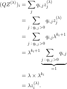
![Rendered by QuickLaTeX.com \[\lambda z_i = \sum_k q_{i,k}z_k = \sum_{k \; : \; q_{i,k}>0} q_{i,k} \underbrace{z_k}_{=\overline{z}} = \overline{z}\underbrace{\sum_{k \; : \; q_{i,k}>0} q_{i,k}}_{=1} = \overline{z}.\]](http://quentin-duchemin.alwaysdata.net/wiki/wp-content/ql-cache/quicklatex.com-467bc10ad7053542f1fe0795344f38d9_l3.png)
Claim 3.3: ![]() is a p-th root of unity.
is a p-th root of unity.
Let us consider ![]() such that
such that ![]() . For all
. For all ![]() , since
, since ![]() , Claim 3.2 gives
, Claim 3.2 gives ![]() and since
and since ![]() (see Claim 3.1), we have that
(see Claim 3.1), we have that ![]() . Hence
. Hence ![]() is an integer and divides
is an integer and divides ![]() . We deduce that
. We deduce that ![]() divides
divides ![]() meaning that there exists some
meaning that there exists some ![]() such that
such that ![]() . We have found that
. We have found that ![]() is a p-th root of unity.
is a p-th root of unity.
Conversely, let us consider ![]() a p-th root of unity. We define the vector
a p-th root of unity. We define the vector ![]() by
by ![]() and
and ![]() if
if ![]() .
.
Claim 3.4: The vector ![]() is well-defined and is an eigenvector associated with the eigenvalue
is well-defined and is an eigenvector associated with the eigenvalue ![]() .
.
![]() We first show that
We first show that ![]() is well-defined. Let us consider some
is well-defined. Let us consider some ![]() . By irreducibility of the matrix
. By irreducibility of the matrix ![]() , there exists some
, there exists some ![]() such that
such that ![]() . Then, for all
. Then, for all ![]() such that
such that ![]() , we have
, we have
![]()
![]()
![]() For all
For all ![]() , we consider some integer
, we consider some integer ![]() such that
such that ![]() . One can easily remark that for all
. One can easily remark that for all ![]() , if
, if ![]() then
then ![]() since
since
![]()
(1) ![]()

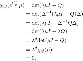
Claim 3.5: Let ![]() be the diagonal matrix with diagonal coefficients
be the diagonal matrix with diagonal coefficients ![]() . It holds
. It holds ![]() . This gives that the eigenvalues associated with the p-th roots of unity of
. This gives that the eigenvalues associated with the p-th roots of unity of ![]() have algebraic multiplicity
have algebraic multiplicity ![]() and the spectrum of
and the spectrum of ![]() is invariant under rotation of angle
is invariant under rotation of angle ![]() .
.
(2) ![]()
![]() Now we prove that all p-th roots of unity are eigenvalues of
Now we prove that all p-th roots of unity are eigenvalues of ![]() with multiplicity 1. Let us consider some p-th root of unity
with multiplicity 1. Let us consider some p-th root of unity ![]() . Denoting for any
. Denoting for any ![]()
![]() the cofactor of some matrix
the cofactor of some matrix ![]() at location
at location ![]() , one can easily check that
, one can easily check that
![]()

![]() Let us consider some eigenvalue
Let us consider some eigenvalue ![]() of
of ![]() . We set
. We set ![]() and
and ![]() the diagonal matrix with diagonal coefficients
the diagonal matrix with diagonal coefficients ![]() . Then,
. Then,

Extension of the Theorem
The Krein–Rutman theorem is a generalisation of the Perron-Frobenius theorem to infinite-dimensional Banach spaces and complex integral operators.
