Davis-Kahan Sin Theta Theorem

In many situations, there is a symmetric matrix of interest $\Sigma \in \mathbb R^{d \times d}$ , but one only has a perturbed version of it $\hat{ \Sigma} = \Sigma + H$ . How is $\hat{ \Sigma}$ affected by $H$ ?
The basic example is Principal Component Analysis (PCA). Let $\Sigma = \mathrm{Cov}(X)$ for some random vector $X \in \mathbb R^d$ , and let $\hat{\Sigma}$ be the sample covariance matrix on independent copies of $X$ . Namely, we observe $X_1, \dots, X_n$ i.i.d. random variable distributed as $X$ and we set

$\hat{\Sigma} := \frac{1}{n} \sum_{i=1}^{n} X_i X_i^{\top}.$

If $X$ is concentrated on a low dimensional subspace, then we can hope to discover this subspace from the principal components of $\hat{\Sigma}$ . How accurate is the subspace we find?

1. Some intuition

An eigenspace of $\Sigma$ is the span of some eigenvectors of $\Sigma$ . We can decompose $\Sigma$ into its action on an eigenspace $S$ and its action on the orthogonal complement $S^{\perp}$ :

$\Sigma = E_0\Lambda_0E_0^* + E_1\Lambda_1E_1,$

where $E_0$ is an orthonormal basis for $S$ (e.g., the eigenvectors of $\Sigma$ that span $S$ ), and $E_1$ is an orthonormal basis for $S^{\perp}$ (this follows from the spectral theorem). We can similarly decompose
$\hat{\Sigma}=\Sigma + H$ with respect to a “corresponding” eigenspace $\hat S$ (with dim $(\hat S) =$ dim $( S)$ ):

$\hat{\Sigma} = F_0\widehat{\Lambda}_0 F_0^*+ F_1 \widehat{\Lambda}_1 F_1^*.$

Suppose we find a few eigenvalues of $\hat{\Sigma}$ that somehow stand out from the rest. For instance, as in PCA, we may find the first few eigenvalues to be much larger than the rest. Let $\hat{S}$ be the corresponding eigenspace. If there is a similarly outstanding group of eigenvalues of $\Sigma$ , then the hope is that the corresponding eigenspace $S$ will be close to $\hat{S}$ in some sense. For instance, we may be interested in how well $\hat{S}$ approximates vectors in $S$ . Any vector in $S$ can be written as $E_0 \alpha$ for some $\alpha \in \mathbb{R}^{\mathrm{dim}(S)}$ , the projection of this vector onto $\hat{S}$ is $F_0F_0^{*}E_0\alpha$ . Then

$\begin{align*} \|E_0\alpha - F_0F_0^* E_0 \alpha\|&= \|(I-F_0F_0^*)E_0\alpha\| \\ &= \|F_1 F_1^*E_0\| \\ &= \|F_1^* E_0 \alpha\| .\end{align*}$

Therefore vectors in $S$ will be well-approximated by $\hat{S}$ if $F_1^*E_0$ is “small”.

The condition we will need is separation between the eigenvalues corresponding to $S$ and those corresponding to $\hat{S}^{\perp}$ . Suppose the eigenvalues corresponding to $S$ are all contained in an interval $[a, b]$ . Then we will require that the eigenvalues corresponding to $\hat{S}^{\perp}$ be excluded from the interval $(a - \delta, b + \delta)$ for some $\delta > 0$ . To see why this is necessary, consider the following example:

$\Sigma := \begin{bmatrix} 1+\delta & 0 \\ 0 & 1-\delta \end{bmatrix}, \quad H:=\begin{bmatrix} -\delta & \delta \\ \delta & -\delta \end{bmatrix}, \quad \hat{\Sigma} := \begin{bmatrix} 1 & \delta \\ \delta & 1 \end{bmatrix}.$

Here, the “size” of $H$ is comparable to the gap between the relevant eigenvalues. Then the eigenvalues of $\Sigma$ are $\lambda_1 = 1 + \delta$ and $\lambda_2 = 1 -\delta$ , and its corresponding eigenvectors are $v_1 = (1, 0)$ and $v_2 = (0, 1)$ . The eigenvalues of $\hat{\Sigma}$ are also $\hat{\lambda}_1 = 1 + \delta$ and $\hat{\lambda}_2 = 1 - \delta$ , but its corresponding eigenvectors are $v_1 = (1/\sqrt 2, 1/\sqrt 2)$ and $\hat v_2 = (-1/\sqrt 2, 1/\sqrt 2)$ , we have $\hat v_2^* v_1=1/ \sqrt 2$ , which can be
arbitrarily large relative to $\delta$ .

2. Distances between subspaces

Let $\mathcal E$ and $\mathcal F$ be $r$ -dimensional subspaces of $\mathbb R^d$ , with $r \leq d$ . Let $\Pi_{\mathcal E}$ and $\Pi_{\mathcal F}$ be projectors onto these two subspaces.
We first consider the angle between two vectors, that is, when $r = 1$ . Then, $\mathcal E$ and $\mathcal F$ are spanned by vectors. Denote the two corresponding vectors as $v_1, v_2 \in \mathbb S^{d-1}$ . The angle between $v_1$ and $v_2$ is defined as:

$(v_1, v_2) = \cos^{-1}\left( v_1^* v_2\right).$

Now, we need to extend this concept to subspaces (when $r > 1$ ). Let $E$ and $F$ be $d\times r$ matrices with orthonormal columns such that range( $E$ ) $=\mathcal E$ and range( $F$ ) $= \mathcal F$ . Then, the projectors can be written as $\Pi_{\mathcal E} =E E^{*}$ and $\Pi_{\mathcal E} =F F^{*}$ .
Now, we define the angle between subspaces $\mathcal E$ and $\mathcal F$ as the following:

Definition
The canonical or principal angles between $\mathcal E$ and $\mathcal F$ are:

$\theta_1 = \cos^{-1}(\sigma_1),\dots , \theta_r = \cos^{-1}( \sigma_r),$

where $\sigma_1, \dots , \sigma_r$ are singular values of $E^* F$ or $F^* E$ .

A general result known as CS-decomposition in linear algebra gives the following:

$E^*F = U \cos \Theta V^*,$

where

$\Theta = \begin{bmatrix} \theta_1 & \dots & 0 \\ \vdots & \dots & \vdots \\ 0 & \dots & \theta_r \end{bmatrix}$

Another way of defining canonical angles is the following:
Definition
The canonical angles between the spaces $\mathcal E$ and $\mathcal F$ are $\theta_k = \sin^{-1}(s_k)$ for $k \in \{ 1,\dots , r\}$ , where $s_1, \dots , s_k$ are the singular values of

$\Pi_{\mathcal E} \left( I - \Pi_{\mathcal F}\right)=E E^*\left( I- F F^* \right) = U \sin \Theta V^*.$

Now, given the definition of the canonical angles, we can define the distances between subspaces $\mathcal E$ and $\mathcal F$ as the following.

Definition
The distance between $\mathcal E$ and $\mathcal F$ is $\|\sin \Theta\|_2$ , which is a metric over the space of $r$ -dimensional linear subspaces of $\mathbb R^d$ . Equivalently,

$\begin{align*} \|\sin \Theta\|_2^2 &=\|\Pi_{\mathcal E} \left( I - \Pi_{\mathcal F}\right)\|_2^2\\&=\|\Pi_{\mathcal F} \left( I - \Pi_{\mathcal E}\right)\|_2^2\\&=\frac12 \|\Pi_{\mathcal E} -\Pi_{\mathcal F}\|_2^2. \end{align*}$

3. Davis Kahan Theorem

Theorem

Let $\Sigma = E_0\Lambda_0E_0^*+E_1\Lambda_1E_1^*$ and $\Sigma+H = F_0\Lambda_0F_0^*+F_1\Lambda_1F_1^*$ be symmetric matrices with $[E_0, E_1]$ and $[F_0, F_1]$ orthogonal matrices. If the eigenvalues $\Lambda_0$ are contained in an interval $(a, b)$ , and the eigenvalues of $\Lambda_1$ are excluded from the interval $(a-\delta, b+\delta)$ for some $\delta > 0$ , then

$\|F_1^*E_0\| \leq \frac{\|F_1^*HE_0\|}{\delta} ,$

for any unitarily invariant norm $\|\cdot\|$ .

Proof.
Since $\Sigma E_0 = E_0 \Lambda_0 E_0^* E_0 + E_1 \Lambda_1 E_1^* E_0 = E_0 \Lambda_0,$ we have

$\begin{align*}H E_0 &= \Sigma E_0 + H E_0 - \Sigma E_0\\&=(\Sigma +H) E_0 -E_0 \Lambda_0 \end{align*}$

Furthermore, $F_1^* (\Sigma+ H) = \hat{\Lambda}_1F_1^*$ , so

$\begin{align*} F_1^*HE_0 &= F_1^*(\Sigma + H)E_0 - F_1^*E_0\Lambda_0\\&= \hat{\Lambda}_1F_1^*E_0 - F_1^* E_0\Lambda_0\end{align*}$

Let $c := \frac{a+b}{2}$ and $r := \frac{b-a}{2} \geq 0$ . By the triangle inequality, we have

$\begin{align*}\|F_1^*HE_0\| &= \|\hat{\Lambda}_1F_1^*E_0 - F_1^* E_0\Lambda_0\|\\&= \|\left(\hat{\Lambda}_1-cI\right)F_1^*E_0 - F_1^* E_0\left(\Lambda_0-cI\right)\| \\ &\geq \|\left(\hat{\Lambda}_1-cI\right)F_1^*E_0 \|-\|F_1^* E_0\left(\Lambda_0-cI\right)\|.\end{align*}$

Here we have used a centering trick so that $\Lambda_0 - cI$ has eigenvalues contained in $[-r, r]$ , and
$\hat{\Lambda}_1 - cI$ has eigenvalues excluded from $(-r -\delta, r + \delta)$ . This implies that $\|\Lambda_0-cI\|_2\le r$ and $\|\left(\hat{\Lambda}_1-cI\right)^{-1} \|_2 \leq \left( r+\delta \right)^{-1}$ , respectively. Therefore

$\begin{align*}\|\left(\hat{\Lambda}_1-cI\right)F_1^*E_0 \| &\geq \frac{1}{\|\left(\hat{\Lambda}_1-cI\right)^{-1} \|_2} \|F_1^* E_0\| \\&\geq \left( r+\delta \right)^{-1} \|F_1^* E_0\|,\end{align*}$

and

$\begin{align*}\|F_1^* E_0\left(\Lambda_0-cI\right)\| & \leq \|\Lambda_0-cI\|_2 \|F_1^* E_0\|\\&\leq r\|F_1^* E_0\|.\end{align*}$

We conclude that $\|F_1^*H E_0\| \geq \delta \|F_1^* E_0\|.$

Another version of the Davis-Kahan Theorem which is more popular in the community of statisticians is the following.

Theorem

Let $\Sigma$ and $\hat{\Sigma}$ be $d \times d$ symmetric matrices with respective eigenvalues $\lambda_1 \geq \lambda_2 \geq \dots \geq \lambda_d$ and $\hat{\lambda}_1 \geq \hat{\lambda}_2 \geq \dots \geq \hat{\lambda}_d$ .
Fix $1 \leq r \leq s \leq d$ , and let $V$ and $\hat V$ be $d \times (s - r + 1)$ matrices with orthonormal columns corresponding to eigenvalues $\{\lambda_j\}_{j=r}^s$ and $\{\hat{\lambda}_j\}_{j=r}^s$ .
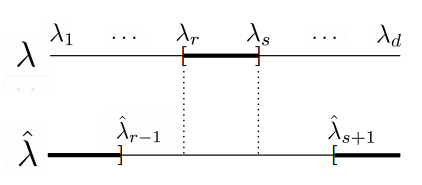
Let $\mathcal E$ and $\mathcal F$ be the subspaces spanned by columns of $V$ and $\hat V$ . Define the eigengap as

$\delta = \inf \left\{ \left| \lambda - \hat{\lambda} \right| \; : \; \lambda \in [\lambda_s , \lambda_r], \; \hat{\lambda} \in (- \infty, \hat{\lambda}_{s+1}] \cup [\hat{\lambda}_{r-1}, \infty)\right\},$

where we define $\hat{\lambda}_0 = -\infty$ and $\hat{\lambda}_{d+1} = \infty$ .
If $\delta > 0$ , then

$\left\|\mathrm{sin} \Theta(\mathcal E, \mathcal F)\right\|_2 \leq \frac{\|\hat{\Sigma}-\Sigma\|_{2}}{\delta}.$

The result also holds for the operator norm $\|\cdot\|_{op}$ .

Illustration of the eigengap $\delta$ . (Source: Alessandro Rinaldo Lecture Notes)

By Weyl’s theorem, one can show that the sufficient (but not necessary) condition for $\delta>0$ in Davis-Kahan theorem is

$\|\hat{\Sigma}-\Sigma\|_2<\min_{r\leq i\leq s, \; j \in [n] \backslash \{r,\dots,s\}} \left| \lambda_i-\hat{\lambda}_j\right|.$

When the matrices are not symmetric, there exists a generalized version of the Davis-Kahan Theorem called Wedin’s theorem.

Perron Frobenius Theorem

2 thoughts on “Davis-Kahan Sin Theta Theorem”

Marylin Ser

September 23, 2023 at 7:46 pm

Reply

Thank you for another informative blog. Where else could I get that type of info written in such a perfect way? I have a project that I’m just now working on, and I have been on the look out for such info.
Dana Blankschan

September 24, 2023 at 6:59 pm

Reply

You really make it seem so easy with your presentation but I find this topic to be actually something which I think I would never understand. It seems too complicated and extremely broad for me. I’m looking forward for your next post, I will try to get the hang of it!

Quentin Duchemin